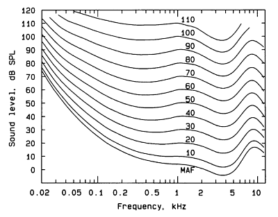

The above graph shows the Equal Loudness Contours, as measured by Robinson and Dadson, 1956. The original measurements were carried out by Fletcher and Munson in 1933, and the curve often carries their name.
The lines represent the sound pressure required for a test tone of any frequency to sound as loud as a test tone of 1 kHz. Take the line marked "60" - at 1 kHz ("1" on the x axis), the line marked "60" is at 60dB (on the y axis). If you follow the "60" line down to 0.5 kHz (500 Hz), and look across to the y axis, the value is about 55 dB. What this means is that a 500 Hz tone at 55 dB SPL sounds as loud to a human listener as a 1 kHz tone at 60 dB SPL.
If every frequency sounded equally loud, then this graph would just be a series of horizontal lines. As it isn't, a filter is required to simulate this characteristic.
Where the lines curve upwards, this means that we are less sensitive to sounds of that frequency. Hence, the filter must attenuate (reduce) sounds of that frequency. The ideal filter will be the inverse of the above graphs. As we don't know the replay level yet, and don't want to use a different filter for sounds of differing loudness, a representative average of the above curves will is chosen as the target filter:
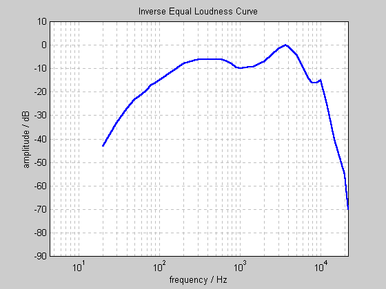
A common approximation to the frequency response of the human ear is the "A" Weighting curve:
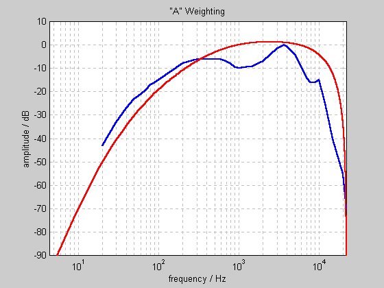
The above graph shows the response of a 2x7 coefficient IIR filter designed to match the A weighting curve. It's only an approximation, and probably not close enough for our purposes. For example, at 15 kHz, the curve lets through 30 dB more energy than the ears of a human listener! The "B" and "C" weighting curves don't get much closer, as the following graph (from this website) shows:
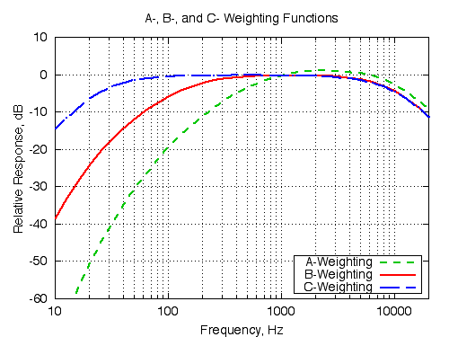
Since none of these standard weighting curves gives a suitable frequency response, a custom filter will be designed, as follows.
MATLAB offers several functions to design FIR and IIR filters to match arbitrary amplitude responses. Feeding the target response into yulewalk.m, and requesting a 2x10 coefficient IIR filter gives the following response:
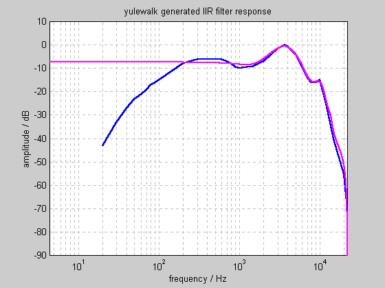
At higher frequencies, this filter is an excellent approximation to our target. However, it lower frequencies, it doesn't even come close. Increasing the number of coefficients does not cause the yulewalk function to perform significantly better.
One solution is to cascade the yulewalk filter with a 2nd order Butterworth high pass filter, with a high pass frequency of 150 Hz. The resulting combined response is close to our target response, and is used by Replay Level:
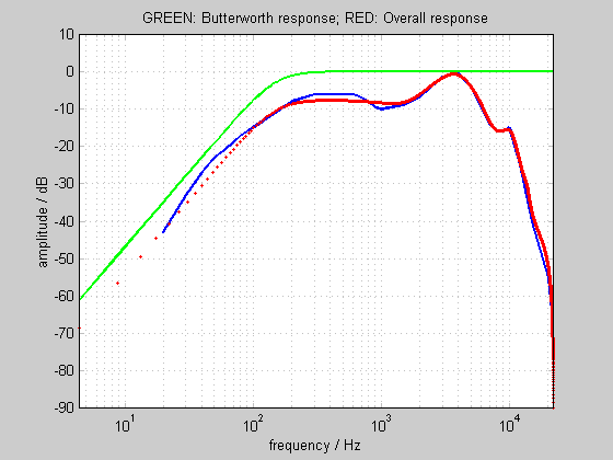
The MATLAB script which generated the above graphs is equalloud.m. It requires adsgn.m to generate the "A" weighting filter for comparison (this file was downloaded from here). The yulewalk and butter functions are built in to MATLAB.
The filter design function called in the MATLAB implementation of ReplayLevel is equalloudfilt.m.
Obviously, if you don't have MATLAB, these scripts and functions aren't much use to you! For this reason, you can download a text doccument containing all the filter coeficients.
As always, suggestions are welcome. The resulting IIR filters are 2x10 and 2x3 coefficients respectively. Someone who is good at filter design may be able to create a single IIR filter of 2x10 coefficients that approaches the target response. If you're willing to do this, please contact me.